An 8.6 GB model that serves only 7 requests a second, and the trace that says why
Part 1 of “The Inference Wall”. One model (Qwen3.5-4B), one mid-range GPU (NVIDIA A10G, 23 GB), measured under real load.
Manas Pathak · August 21, 2026
The Inference Wall · All posts · Part 1
Say you want to run an open-source language model yourself instead of calling an API: you rent one GPU, download the model’s weights onto it, and start a server that answers requests. This is called self-hosting, and the practical question everyone asks first is “how many requests can one GPU handle at once?” The intuition most people carry is that it comes down to whether the model fits: if the weights fit in the GPU’s memory with room to spare, you should be in good shape.
I put that intuition to the test, and it was badly wrong. Here is the experiment. I took Qwen3.5-4B, a mid-size open model whose weights occupy 8.6 GB, and loaded it onto a mid-range GPU with 23 GB of memory. It fit easily, using about a third of the GPU, with 14 GB to spare. Then I sent it a growing stream of requests, raising the arrival rate step by step, and watched for the point where the server stopped keeping up: where requests arrived faster than it could finish them, so a backlog began to build.
That happened at about seven requests per second.
Not seven thousand. Seven. A whole modern GPU, a model that fits with room to spare, and it saturates at a single-digit request rate. The lesson, which the rest of this post unpacks: “does it fit in memory” tells you almost nothing about how much traffic a GPU can serve. Memory was never the bottleneck here; something else ran out first. I will show you how to see that ceiling in a latency curve, work out what the GPU is actually spending its time on, and then open a profiler trace to confirm it.
If the terms KV cache, prefill, or decode are new, the primer (“How an LLM actually serves a request”) builds the whole picture first; this post assumes it. You do not need to have run a GPU yourself; if you have deployed a service behind an API and rented GPU capacity from a cloud provider, you are the reader this is for.
The setup, stated loudly so you can argue with it
- Model:
Qwen/Qwen3.5-4B, served text-only, in fp16 (each weight stored as a 16-bit number, the default full-precision format; the quantization post swaps in a 4-bit version). It is a hybrid-attention model: only 8 of its 32 layers keep a growing KV cache, the other 24 use fixed-size state. That detail keeps KV memory cheap and recurs throughout, so it is worth flagging up front. - GPU: a single NVIDIA A10G (Ampere, 23 GB usable).
- Server:
vllm serve(vLLM 0.18.0), CUDA graphs on,max_num_seqs=256,gpu_memory_utilization=0.9. - Workload: every request is 256 input tokens and 128 output tokens, with
--ignore-eosso every request emits exactly 128 tokens. Fixed, so nothing hides in length variance. - Load:
vllm bench serve, a tool that fires requests at a chosen rate and records how long each one took. It reports three latencies, and it is worth knowing what each one means because they tell different stories:- TTFT (time to first token): how long you wait after sending a request before the first word of the answer appears. This is the “is it responding?” feeling.
- ITL (inter-token latency): once it starts, the gap between each streamed word. This is the “is it typing smoothly?” feeling.
- E2E (end-to-end): total time for the whole answer. Each is reported at percentiles (p50 = the median request, p99 = the worst 1%), because averages hide the tail, and the tail is where users get angry. “Throughput” is the separate question of how many requests (or tokens) the server clears per second.
One thing before any numbers: every measurement below is from a warm server. The very
first request at rate 1 reported a median TTFT of 98 ms but a p99 of 29,272 ms, a 300x
gap on an unloaded server. That is not queueing. The first time the server sees a given
batch size it pauses to build optimized GPU code for it (torch.compile compiles the model’s
operations, and vLLM captures a CUDA graph, a replayable recording of the GPU work), a
one-time cost that lands entirely in the tail. Re-run the same point warm and it drops to
median 95 ms, p99 138 ms, a 200x collapse. So the procedure behind every number here is: run
the whole sweep once to pay those costs, throw that pass away, and measure the second. One
warm-up request is not enough, because the cost is paid per batch size; only running the
full sweep first touches every batch size the measured pass will hit.
Where the memory went (and why it is not the story)
Before hitting it with load, look at how vLLM carves up the 23 GB between the two things from the primer: the fixed model weights and the growing KV cache. vLLM reports the split at startup (numbers quoted from its log, not my arithmetic):
- Model weights: 8.61 GiB.
- Available KV cache: 9.45 GiB, which is 77,088 tokens.
- Max concurrency at 2,048 tokens per request: 83.7x.
That concurrency figure is surprisingly generous, thanks to the hybrid-attention design: with only 8 of 32 layers growing a cache, each request’s real footprint is far smaller than its token count suggests, so vLLM’s planner fits about 2.2x the naive 77,088 / 2,048 = 37.6. (That same ~2.2x discount reappears in the quantization post’s 9B numbers.) What the line means is the point: the cache has room for 83 max-length requests at once, hundreds on the short 256/128 workload, and the server never runs more than a handful concurrently. It comes nowhere near filling the cache. So when it tops out at seven requests a second, it did not run out of room to remember conversations. It ran out of something else.
The curve: flat, then a knee, then a cliff
Here is the sweep on the warm server. The first column is the rate we send requests at; the second is the rate the server actually completes them. Watch how they diverge, and watch the p99 tail.
| Requested rate | Completed req/s | Output tok/s | TTFT p50 | TTFT p99 | E2E p99 |
|---|---|---|---|---|---|
| 1 /s | 0.99 | 126 | 96 ms | 138 ms | 3,153 ms |
| 2 /s | 1.95 | 249 | 101 ms | 173 ms | 3,538 ms |
| 4 /s | 3.77 | 482 | 128 ms | 216 ms | 4,786 ms |
| 6 /s | 5.41 | 693 | 198 ms | 402 ms | 8,031 ms |
| 8 /s | 6.37 | 815 | 386 ms | 789 ms | 17,869 ms |
| 10 /s | 6.22 | 796 | 556 ms | 6,949 ms | 21,360 ms |
| 16 /s | 7.05 | 902 | 793 ms | 11,359 ms | 19,969 ms |
| 32 /s | 8.20 | 1,049 | 2,279 ms | 13,642 ms | 19,391 ms |
| inf (flood) | 8.53 | 1,092 | 5,030 ms | 18,877 ms | 23,422 ms |
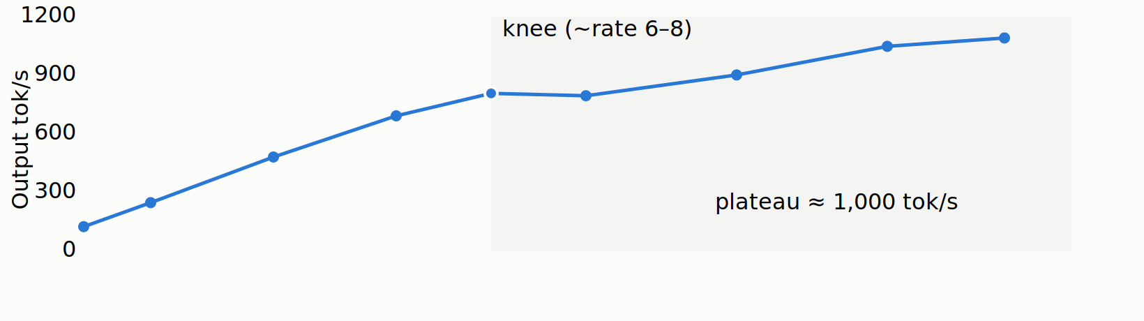
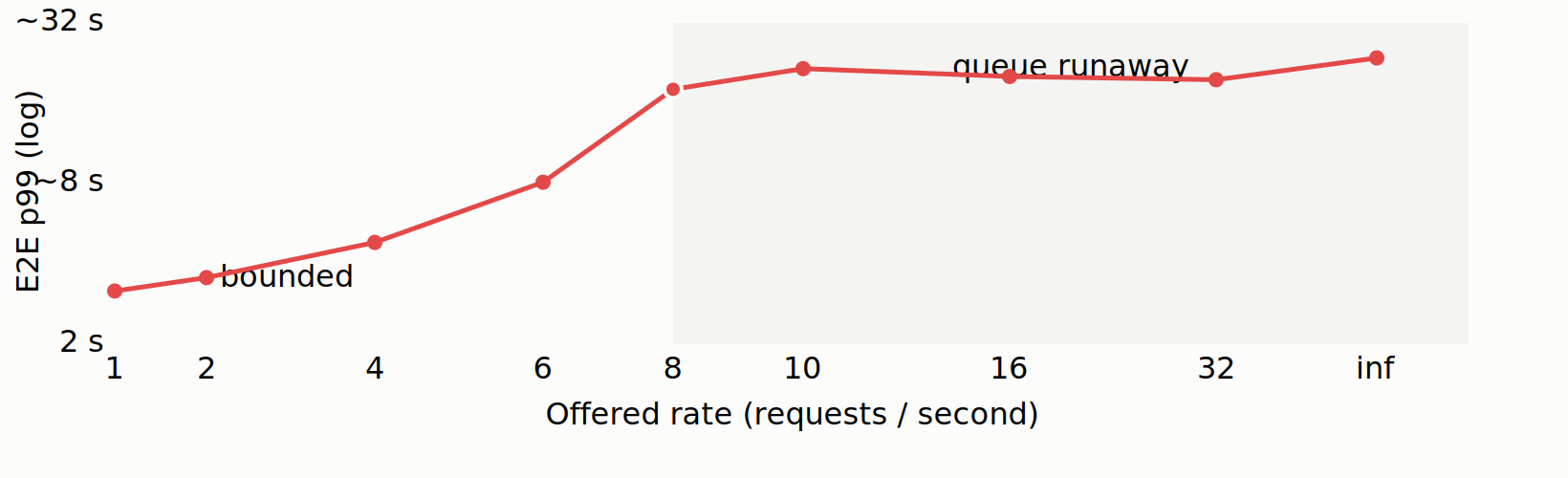
One shape, three regimes, and you will see it on every serving system you load-test. Below rate 6 the completed rate tracks what you send (offer 6, get 5.4) and the tail stays bounded (E2E p99 under 8 s): this is where you want to operate. Around rate 6 to 8 the ceiling arrives, completed throughput flattens at 7 to 8.5 req/s and sending more stops helping. Past that, requesting 10, 16, 32, or infinity all land on the same ceiling while the p99 TTFT runs away (402 ms at rate 6, 6,949 ms at rate 10, 13,642 ms at rate 32). That runaway is the queue: requests arrive faster than the server completes them, so a backlog builds and each one waits longer behind it. Why the server caps at seven or eight a second, no matter how many you send, is the next section.
The wall is decode, not memory capacity
So what is the ceiling made of, if not memory? The KV cache has room to spare, so the answer is the decode loop. Recall the machine from the primer: each step streams all 8.6 GB of weights from memory once and, with that single stream, advances every request in the batch by one token. The ceiling is how fast that stream can happen, repeated once per token.
Put a number on it with a single request, no batch to hide behind. Each output token costs about 20 ms. That is not the arithmetic: one token is roughly 8.6 billion operations, which the A10G’s 66 TFLOP/s does in about 0.13 ms. It is the weight-stream. The A10G moves about 483 GB/s (I measured it by timing a large on-GPU copy), and the 8.61 GiB of weights is ~9.2 GB, so one stream takes about 19 ms, essentially the whole 20 ms. The token time is the weight-streaming time. Hitting this limit is called being memory-bandwidth bound, and it is the floor every request pays.
Batching is what lifts you off that floor: one 19 ms stream advances the whole batch, so throughput climbs from 126 tok/s at a single request toward ~1,090 tok/s under load. But it does not climb forever. Each request also carries its own un-shareable work in the step (attending to its own KV cache), and once the batch is big enough that this per-request work, not the shared stream, fills the step, adding requests stops buying throughput. On this model that plateau lands around a batch of 64, and the server settles at ~1,090 tok/s. At 128 output tokens per request that is about 8.5 requests a second under a full flood, the same seven-to-eight wall the curve showed, and the GPU is neither idle nor out of memory when it hits it. (Part 3 pins down exactly where the plateau sets in.)
This also explains the queue from the curve above. The running batch is load-driven, not the
max_num_seqs=256 ceiling: about 1 request at rate 1, and ~145 under a flood. Past the
batch-64 plateau those extra in-flight requests buy no more throughput, they just wait their
turn, and that waiting is the tail latency blowing up.
Which limit you hit changes with model size
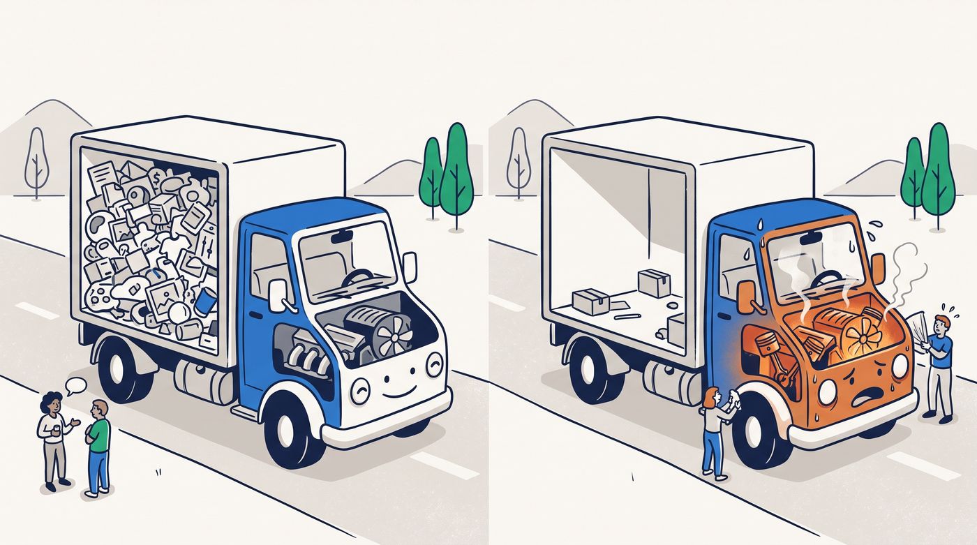
Here is the part worth internalizing, because the answer flips with model size and it is the crux of capacity planning.
- On a tiny model (say a 0.5B), the weights are only about 1 GB, so streaming them each
step is quick and generation speed is not the problem. What runs out first is memory: the
KV cache or the
max_num_seqscap fills up while the GPU still has compute to spare. - On this 4B, it is the mirror image. The hybrid-attention design leaves KV memory abundant (the 83-request budget the workload never touches), so memory is not the limit; generation speed is. Every decode step has to stream 8.6 GB of weights from memory, and that streaming is slow enough that the server cannot clear more than seven or eight of these requests a second, long before memory is tight.
Same GPU, same test harness, opposite limit, purely because the model got bigger. This is why “does it fit” is the wrong first question. It fits fine. The right question is “which limit do I hit first under load,” and the answer is not visible in a memory report. You have to put the server under load and watch the curve.
Reading it off a trace
The arithmetic above says the server is saturated; a profiler trace lets us watch it happen.
A trace records every piece of work the GPU runs as a kernel (one unit of GPU work, like a
single matrix multiply) on a timeline. vLLM can turn its profiler on while serving; I did, and
opened the result in chrome://tracing (it ships with this post). During decode the timeline
shows the same kernels running back to back with no gaps: the instant the GPU finishes one
token it starts the next. That is a saturated GPU, no idle time to reclaim and no bubble to
optimize away.
One honest limit: gap-free kernels prove the GPU is busy, not what it is busy on, a weight-streaming bottleneck and an arithmetic one look equally packed. That verdict came from the arithmetic (token time matching the 19 ms stream), not the picture. What the trace rules out is a stall or idle gap, so the only levers left are the ones that change how many bytes each token reads (quantization, a later post) or how work is scheduled around big prefill lumps (chunked prefill, next post).
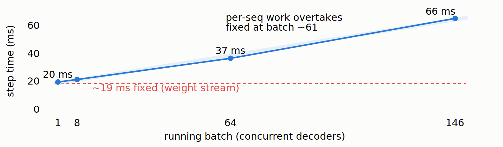
I later profiled steady decode directly at several batch sizes to check the model above, and
it holds almost exactly. The per-step time fits 19.1 ms + 0.31 ms x batch: a fixed ~19 ms
(the shared weight stream, matching the 19 ms floor from the arithmetic) plus a per-sequence term that only starts
to dominate around a batch of 61, which is the plateau this post has been calling “around 64.”
The GPU is 97 to 99.7% busy throughout, no idle gap to reclaim. The traces also forced a
correction: pure decode with no new arrivals reaches ~2,200 tok/s, about twice the ~1,090
the server sustains in practice. The difference is prefill: under real load, incoming prompts’
prefill competes for the same steps and eats roughly half the GPU (the subject of the next
post). So ~1,090 tok/s is the serving ceiling; the raw decode ceiling is higher, and prefill
is what stands between them.
What to take away
- “It fits” tells you nothing about throughput. An 8.6 GB model on a 23 GB GPU, two-thirds empty, still capped at ~7 req/s. Memory headroom and serving capacity are different resources.
- Load-test to find the knee, and operate below it. The flat regime (here, up to about rate 6) is where latency is bounded. Past the knee you buy nothing but queue. The knee is invisible in any single-request benchmark; you only see it under a rate sweep, reported in percentiles.
- Know which limit you hit first, because it changes with model size. A server has several limits (memory to hold requests, speed to generate tokens), but only one caps you under load. On a small model it is usually memory; on a bigger one like this 4B it is generation speed. The fix differs for each, so diagnosing which one you are in is the job.
- Warm the server before you believe any number. The cold p99 was 200x the warm one. Publish the cold number and you are describing a server nobody runs.
Next in the series: the same 4B model, but now we inject a big prompt into a stream of short ones and watch it freeze the decoders, then flip one flag and watch the freeze shrink by 2.4x, with the trace that shows the stall happening kernel by kernel — Part 2.
Reproduce: the sweep and probe scripts are in
experiments/01-hit-the-wall/
(server launch scripts in
scripts/); the raw
sweep logs, the startup memory report, and the captured decode traces (openable in
chrome://tracing) are in
benchmarks/01-hit-the-wall/.
The rig is a single A10G; your absolute numbers will differ, the shape will not.
Previous: Primer: how an LLM serves a request · Next: Part 2: The prefill freeze · All posts
Disclaimer: This blog is written and published in my personal capacity. The opinions, findings, and conclusions expressed herein are solely my own and do not necessarily represent the views, policies, or endorsements of my current or past employers.