The attention sink: why deep layers fixate on the first token
Part 4 of “The Inference Wall”. A detour from the usual rig: instead of Qwen3.5-4B under load on an A10G, this one opens up a small model, GPT-2, on a CPU, keeping every intermediate value so the arithmetic is slow enough and small enough to read.
Manas Pathak · September 18, 2026
The Inference Wall · All posts · Part 4
Most of this series watches models from the outside. How many tokens per second, how big a batch, how the work looks in a profiler trace. That’s the serving layer, the plumbing that turns your prompt into an answer fast, and it’s where the money is.
But there’s a layer underneath that the plumbing never shows you: the actual thinking. When a model reads your prompt, it does a huge pile of arithmetic. Which earlier tokens does it look at? How strongly? What is it holding onto as it goes? Those numbers exist for a fraction of a second and then they’re gone.
For one prompt, you can capture all of it: every attention weight and every intermediate state the model computes as it reads. On a small model, two effects stand out, and they turn out to be two sides of one phenomenon that sits under a real problem in serving these models cheaply.
What attention is doing
If you’ve read the primer on what happens inside an LLM, skip ahead. If not, take one sentence: The cat sat on the keyboard again. The model reads it one token at a time; for simplicity, let’s say each word is a token. When it reaches “sat” it has a problem. On its own, “sat” is unresolved: the thing that sat is back at “cat.” To resolve it, the model reaches back over the tokens it has already read and pulls “cat” toward “sat.” That reaching back is attention, and it is the whole reason a model handles a sentence rather than an unordered pile of tokens.
It doesn’t attend to just one earlier token. Each token spreads a fixed budget of weight across every token from the start of the sentence up to and including itself: non-negative weights that sum to 1, a probability distribution. It can’t look ahead, only back and at itself. Each weight is the slice of attention that one token hands to another. When the model processes “sat,” a well-behaved distribution puts most of its weight on “cat” and a little on “the,” with some kept on “sat” itself.
And the model does this many times over in parallel. Each pass is a head, and different heads look for different things: one might chase the subject of the verb, another just the token right before. Stack those heads into layers that refine the picture, and a small model already holds a lot of them. GPT-2, the one I’ll use here, has 12 layers of 12 heads: 144 separate weight distributions for every token. It’s old and small, but the mechanism is the one today’s models still run. Grouped-query attention and rotary embeddings change how many key-value heads there are and how position is encoded, not the basic act of spreading a normalized budget over the tokens in view, and the artifacts I’m about to show up in current models too. That was the thing I wanted to see.
Getting the numbers out
The fast tools everyone serves models with, like vLLM or Ollama, can’t show you this: they
compute the answer and discard the intermediate numbers. To see them you use a slower library,
HuggingFace transformers, and ask it to hand back what the fast tools throw away.
If you don’t care about the code, skip the gray boxes. It comes down to three settings that mean keep the attention weights, keep the running state, and keep the memory of earlier tokens:
model = AutoModelForCausalLM.from_pretrained(
    "gpt2", attn_implementation="eager", torch_dtype=torch.float32,
).eval()

out = model(**enc,
            output_attentions=True,      # keep the attention weights
            output_hidden_states=True,   # keep the running state at every layer
            use_cache=True)              # and the memory of earlier tokens (the KV cache)
That gives back two things worth staring at. The attention weights: for my eight-token
sentence, a stack of 8x8 grids, one per head, where each row is a token and each cell says how big
a slice it gave to a token at or before it. And the running state: the vector the model carries
for each token, snapshotted after every layer. The full runnable version is
observe.py.
What one head is looking at
The clean way to read an attention grid: pick a row, which is one token, and the bright cells are
the earlier tokens it leaned on. I picked "The cat sat on the keyboard again." because some heads
do something genuinely readable with it.
Take layer 4, head 3. It’s a subject-tracking head: several later tokens reach back and grab the subject of the sentence. “sat” looks at “cat” with a slice of 0.96, “on” looks at “cat” at 0.89, even the final period points back at “cat.” You can watch the model tie the sentence together, exactly the intuition you’d hope for. Now score every head by a different number: how big a slice does the last token hand to the first token? One head wins outright. Layer 5, head 1 gives the first token a slice of 1.00, its whole attention. Here the two sit side by side:
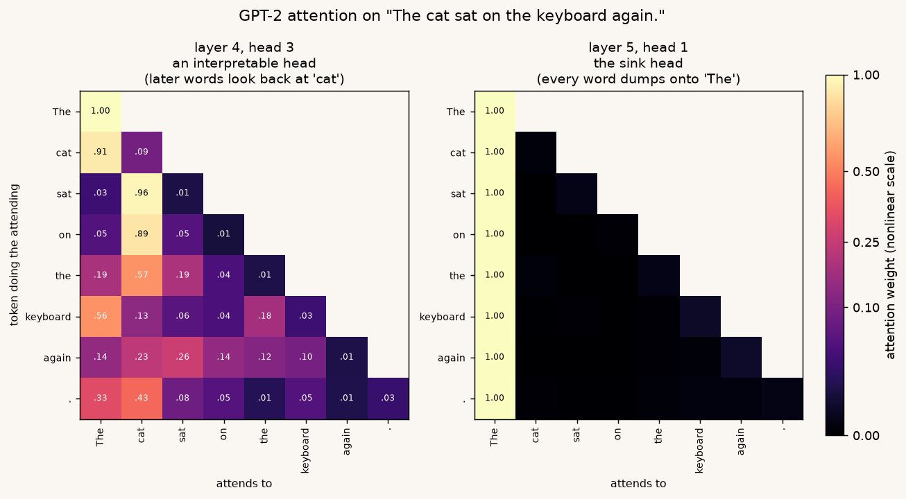
Each row is a token doing the looking; each cell is the slice it gave a token it can see, meaning an earlier one or itself. Numbers are printed in, darker means smaller, and the blank upper triangle is just the future, which no token is allowed to see. Left, layer 4, head 3: a readable head, where later tokens reach back to the subject, “cat.” Right, layer 5, head 1: every token, whatever it means, hands its entire slice to the first token, “The.”
The left panel is what I assumed all attention looked like: tokens wiring up to each other, meaning getting assembled. The right panel is the surprise. A whole head, deep in the network, has decided the single most useful place to look is a throwaway article at the front of the sentence.
And it isn’t one odd head. If I score all 144 by that same first-token measure and lay them out as a grid, the back half of the network lights up almost entirely:
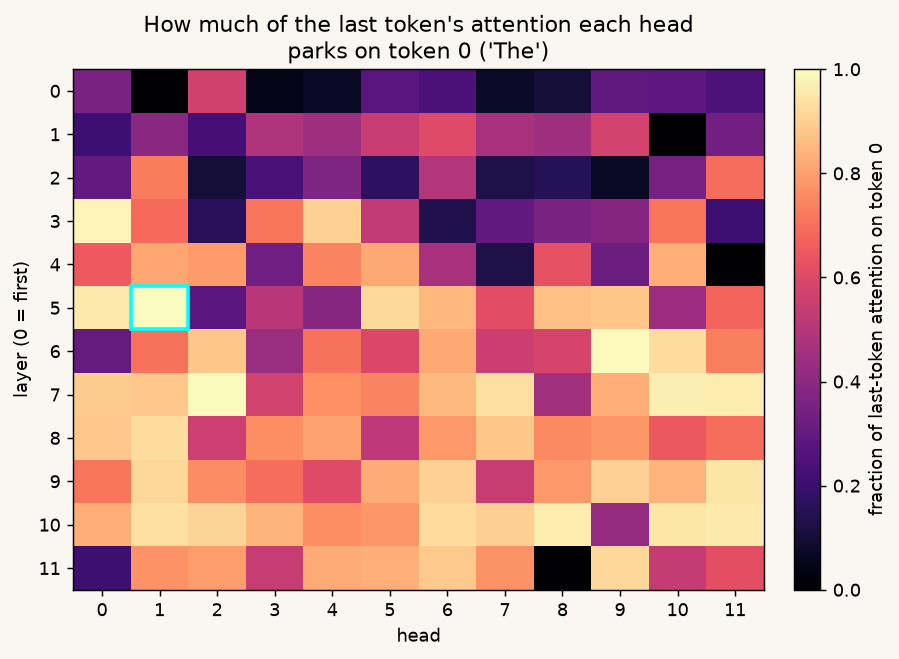
Each square is one head, shaded by how much of the last token’s attention it sends to the first token. The early layers up top still do real local work like the subject-tracking head above. Deeper in the network, most heads have gone bright. The boxed square is layer 5, head 1. Across the back half of the network, 92% of heads send more than half their attention to the first token.
Why the sink forms
This is a known effect, called an attention sink, and once you see the reason it stops being mysterious.
The mechanism is the softmax. It gives every visible token a positive weight and forces the total to exactly 1, so a head has no way to say “none of these tokens matter to me right now.” Each head computes one specific relation between tokens; when that relation is simply absent from the current sentence, the head has nothing informative to point at, yet it still has to emit a full distribution. It has to spend that weight somewhere.
The cheapest place is a token that is always present, always in the same spot, and carries no meaning worth disturbing: the first one. The sink is where a head offloads attention it has no use for, a safe, always-available target. The first token gets the job because every later token can see it, and a fixed target is easy for the model to learn. Over training the model comes to rely on that escape valve: the weight a head has nowhere else to put has a reliable place to go. The StreamingLLM paper by Xiao et al. in 2023 named this effect and showed that the model depends on it — which is precisely why, as we will see, you cannot simply delete those first tokens from a long context without breaking the model.
The second effect: one token’s magnitude explodes
While I had the internals open, I looked at the other thing the model hands back: the running state it carries for each token. Each token’s state is a vector, and I can summarize it with a single number: its magnitude, the plain length of that vector, its L2 norm: the square root of the sum of its squared components. Every token’s vector has the same number of components, 768 of them in GPT-2, so this isn’t about one token having a longer vector than another. It’s about how big the numbers inside are. For each token I take the largest magnitude it reaches at any layer. Seven of the eight land within a narrow band. One does not.
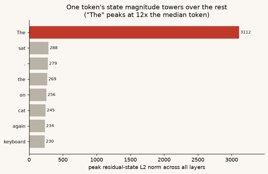
Each bar is one token’s largest internal-state magnitude across all layers. Seven tokens sit in a tight band near a magnitude of 250. “The” reaches about 3,100, roughly 12 times the median token. That single value is large enough to dominate everything the network carries at that position.
The outlier is the first token again. Its magnitude also climbs highest in the middle layers and eases back toward the pack by the final one, so if you only read the model’s output, which is all you normally get, you’d never see it. You have to look inside the computation to catch it.
These spikes are called massive activations, named by Sun et al. in 2024, and they’re almost certainly the same mechanism as the sink seen from the other side. The research argues the model parks a big, roughly constant value on the first token, and it’s that value the spare attention keys onto: the token that soaks up the leftover attention is the same one carrying the outsized magnitude.
I ran the same check across a handful of other models, including Meta’s OPT (Open Pre-trained Transformer, an early open-source LLM family) and Alibaba’s Qwen, and both effects showed up every time. GPT-2 is just the clearest place to see them.
Why the fast tools can’t show you this
I found all of this without touching vLLM or Ollama, the tools I use everywhere else, because they never build the picture I just showed you.
That 8x8 grid, one weight for every pair of tokens, is the expensive part of attention. For a real prompt of thousands of tokens it’s a grid of millions of cells, and its size grows with the square of the length. The entire art of fast serving is to get the result of attention without ever writing that giant grid down. FlashAttention, the subject of a coming post, computes it in small tiles and never stores the full grid. PagedAttention, the trick vLLM is built on, is the other half: it keeps each request’s earlier-token memory scattered across fixed-size blocks rather than in one neat contiguous table. Between them the full grid is never assembled and the memory behind it is never laid out for you to read. Speed comes precisely from throwing away the scratch work I wanted to read.
The numbers I plotted exist for only a few microseconds inside a fused chip operation and then they’re gone. The serving layer stays perfectly observable, and watching it is most of what this series does. But this deeper math layer is deliberately optimized out of existence in the fast path. To see it, you run the slow version: one small model, full precision, on a CPU, with the flags that keep everything. It would never survive in production. It’s also the only version that stops to write down what the model is thinking.
Why it matters
The sink is not just a quirk of an eight-token sentence: it sits under one of the hardest problems in running these models cheaply.
The sink is why you can’t just forget the start of a long chat. When a conversation runs past a model’s window, the obvious fix is to drop the oldest tokens. StreamingLLM showed this wrecks the model’s quality, and the sink is why: the deep layers are still pouring most of their attention onto those first few tokens. Delete them and every head’s attention has to be re-slid onto tokens that were only ever meant to be ignored, and the model falls apart. The fix is to always keep the first few tokens in the window, no matter how long the conversation grows, so the sink never disappears from under the deep layers.
The two effects are one phenomenon seen from two sides. A large, roughly constant value sits on the first token, and the model’s spare attention drains onto it. Neither has anything to do with the word “The” in particular; the first token is simply a convenient, always-present place to park what the model doesn’t need. That bookkeeping is not a curiosity. It sets a hard limit on one of the nastiest problems in serving these models: what you can evict from a long context.
Method: GPT-2, HuggingFace transformers eager attention, full precision, CPU, prompt
"The cat sat on the keyboard again." The sink score is the last token’s attention weight on the
first token, per head. The magnitude spike is the largest per-token state vector magnitude, its L2
norm, relative to the median, across all layers. The code that produces both figures lives in
experiments/04-attention-internals/:
observe.py pulls the weights and running state out of the model, and plot.py renders the three
figures above. No GPU needed; it runs on a CPU in a few seconds.
Previous: Part 3: The batching cliff · Next: Part 5: Starving the cache · All posts
Disclaimer: This blog is written and published in my personal capacity. The opinions, findings, and conclusions expressed herein are solely my own and do not necessarily represent the views, policies, or endorsements of my current or past employers.